
Chua's Circuit
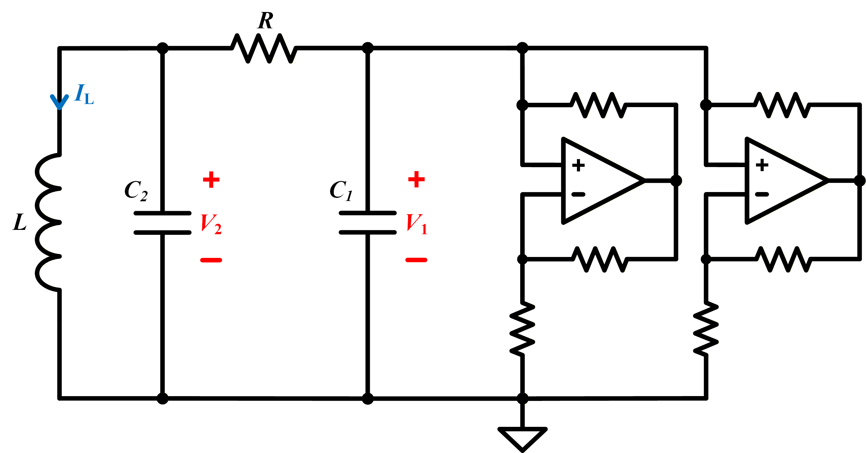
Back in the early days of chaos theory, researchers who wanted to use their mathematical models in the real-world would build analog circuits (called chaotic circuits) to generate unpredictable electrical signals that followed simple equations. One of the applications being investigated was to encrypt messages within these signals, making them undecipherable unless you knew the equations themselves.
The problem was that if your model had a simple multiplication operation, its corresponding circuit implementation was likely to fail because the analog multipliers that could multiply two electrical signals were unreliable at the the time. This is why a professor named Leon Chua set out to find a better way and came up with what we call Chua’s circuit, a simple circuit that uses a few passive components (resistors, capacitors and an inductor) and two op amps.
This circuit is straightforward and inexpensive to build for anyone with some basic experience in electronics and there are several great tutorials out there on how to generate a chaotic attractor from it. But understanding how this circuit works is another story as there aren't many resources that walk through how Leon Chua came up with it. That's why in this blog, I'll follow the classic papers by Kennedy (1993a, 1993b) to show how Chua's circuit naturally evolves from the basic RLC circuit that gets covered in undergraduate physics to the final circuit.
RLC circuit
We'll start with a basic parallel RLC circuit:
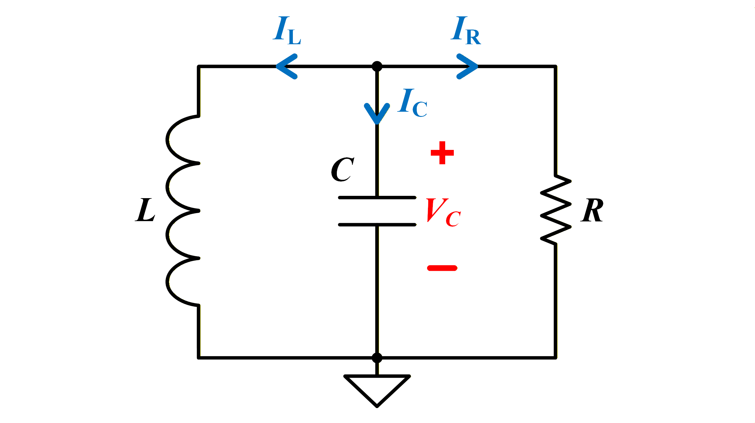
which has the following state equations from KCL and KVL equations:
$$\begin{aligned}\dot{I}_L &= V_C/L, \\\dot{V}_C &= -(V_C/R + I_L)/C.\end{aligned}$$
This circuit oscillates briefly when underdamped and its voltages and currents go to zero, like a car slamming on its brakes and rocking back and forth. We can analyze this by finding the fixed point of this system where the voltages and currents are zero, and then determining its stability which determines how the trajectory (the voltages and currents) will evolve near that point.
To find the fixed point, set the time derivatives equal to zero by setting $\dot{I}_L = 0$ and $\dot{V}_C = 0$, and then solve for $I_L$ and $V_C$, which gives you the system's only fixed point at $(I_L, V_C) = (0,0)$. Then to find the stability of that fixed point, first rewrite the system in state-space form:
$$\frac{d}{dt}\begin{bmatrix}I_L \\V_C\end{bmatrix}=\begin{bmatrix}0 & \frac{1}{L} \\-\frac{1}{C} & -\frac{1}{RC}\end{bmatrix}\begin{bmatrix}I_L \\V_C\end{bmatrix}$$
And then calculate the eigenvalues of its state matrix:
$$A = \begin{bmatrix} 0 & \frac{1}{L} \\ -\frac{1}{C} & -\frac{1}{RC} \end{bmatrix}.$$
$$\det(A-\lambda I)=0 \quad \Rightarrow \quad \lambda^2 + \frac{1}{RC}\lambda + \frac{1}{LC}=0$$
Solving gives:
$$\lambda_{1,2} =-\frac{1}{2RC}\pm\sqrt{\left(\frac{1}{2RC}\right)^2 - \frac{1}{LC}}.$$
where $\lambda_{1,2} = -5000 \pm j31{,}225$ if we pick parameters $R = 1000\,\Omega$, $C = 100\,\text{nF}$, and $L = 10\,\text{mH}$.
These eigenvalues are part of the system’s general solution that describe how the trajectory (the voltages and currents) evolve over time. We can determine the stability by looking at their sign: if the eigenvalue is negative, the voltage and current will decay over time, and if they are also complex, the signals will oscillate as they decay. Additionally, each eigenvalue has a corresponding eigenvector $v_{1,2}$, which identifies a direction of motion. You can read more about eigenvectors and the different types of fixed points in Chapter 5 of Strogatz (2015).
Setting the capacitor voltage to start at $V_C(0)=1\,\text{V}$, the inductor current at $I_L(0)=1\,\text{mA}$, and solving the equations numerically, the system evolves as shown:
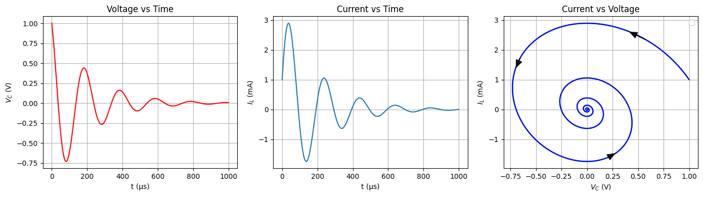
This circuit cannot sustain oscillations because the resistance acts as "friction" and causes the voltage and current to eventually decay toward the fixed point. One way to sustain these oscillations is to have a hypothetical resistor that adds energy to the circuit. For example if we were to make $R \to -R$, the real part of the eigenvalues become positive and the trajectory grows by spiraling out from the origin instead of decaying:
.png)
If we had such a hypothetical resistor we could put it in series with the actual resistance of our parallel RLC circuit to cancel the resistance out.
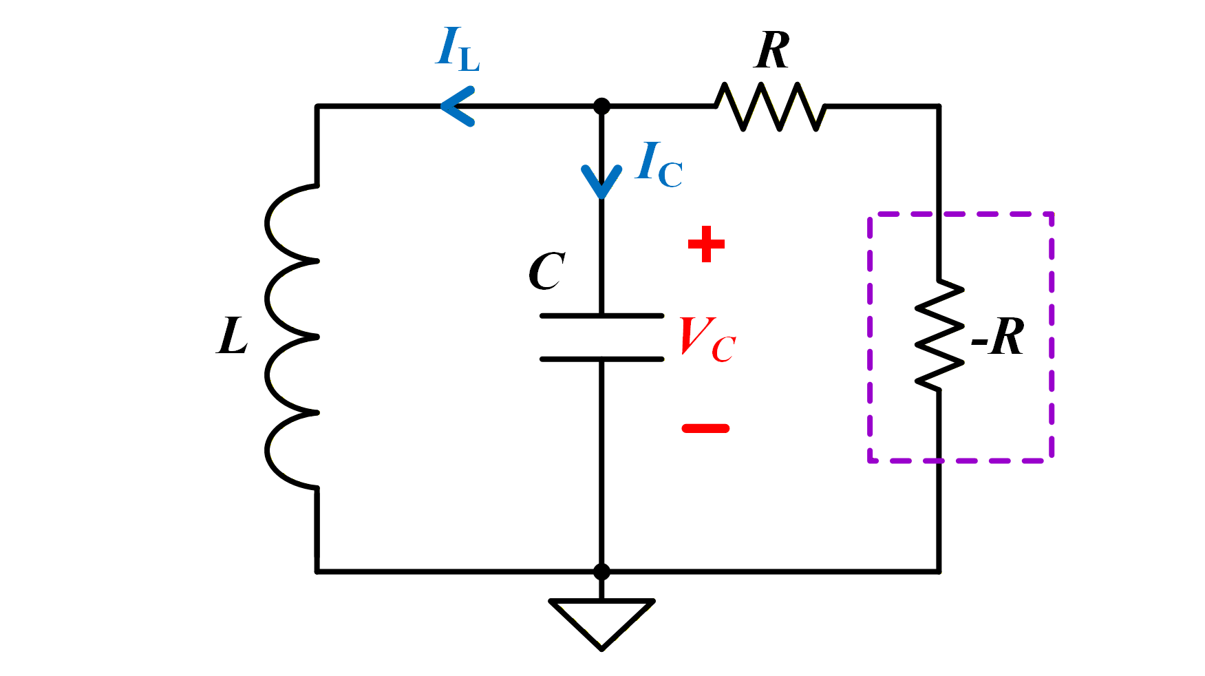
Our negative resistor $R$ would ideally have a linear I-V curve with a slope of $-1/R$ (or conductance $-G$).

Of course, resistors that infinitely add energy don't exist, but there are circuits that simulate a negative resistance in a region. One such circuit is called a negative impedance converter which implements $R = -R_{1}R_{2}/R_{3}$, a negative resistance.
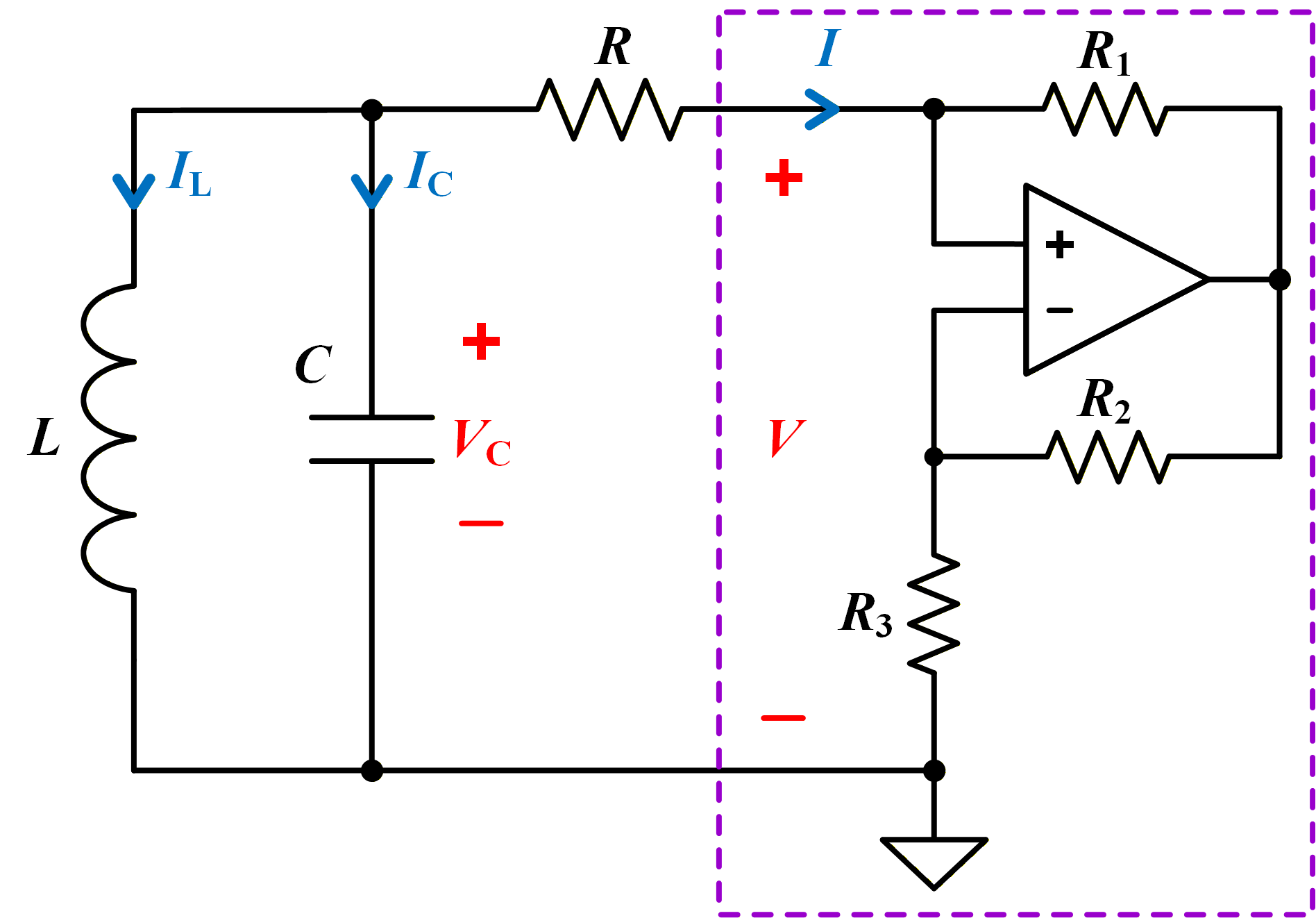
A negative impedance converter is not a perfect negative resistor though, and at some point the output voltage of the operational amplifier will reach the maximum power supply voltage $V_{sat}$. When this happens, the circuit transitions from a resistor with a negative conductance of $G_a$ to a resistor with a positive conductance of $G_b$:

Calculating the slopes through the op amp rules, KCL, and KVL yields a piecewise-linear I-V characteristic:
$$I(V) =\begin{cases} G_b V + (G_b - G_a)E, & V \le -E \\ G_a V, & |V| \le E \\ G_b V + (G_a - G_b)E, & V \ge E \end{cases}$$
where $G_a < 0$ is the negative slope in the central region and $G_b > 0$ is the positive slope in the outer regions. To calcuate the breakpoints, set the output of the op amp to $V_{sat}$, and use the voltage divider of $R_2$ and $R_3$ to obtain $E = \pm V_{sat}[R_2/(R_2 + R_3)]$, which is the voltage across the negative impedance converter when it saturates.
Adding the second capacitor
This circuit is starting to look similar to Chua's circuit except it has one capacitor instead of two. It turns out that we have to add the second capacitor by necessity because otherwise you cannot model this circuit's full behavior. We start by writing out the equations of the circuit so far with one capacitor:
$$\begin{aligned}\dot{I}_L &= V_C/L, \\\dot{V}_C &= -[(V_C - V)/R + I_L]/C.\end{aligned}$$
$$I(V) =\begin{cases} G_b V + (G_a - G_b)E, & V \le -E \\ G_a V, & |V| \le E \\ G_b V + (G_a - G_b)(-E), & V \ge E \end{cases}$$
We also have the following condition from Ohm's Law across resistor $R = 1/G$,
$$I(V) = (V_C - V)/R$$
Following the example of the RLC circuit, we go through the same calculation to find the fixed points by setting derivatives to zero, solving for $I_L$ and $V_C$ and finding the type of fixed point through the eigenvalues. We can additionally solve for $V$ using the previous condition. Note that there are two regions to analyze (when $|V| \leq E$ and $V \geq |E|$) due to the piecewise-linear equation. After tedious algebra we get the following fixed points:
Middle segment: When $|V| \leq E$, where $I(V) = G_a V$ the fixed point and the eigenvalues are:
$$(V, V_C, I_L)=(0, 0, 0)$$
$$\lambda = -G_a^"/2C \pm \sqrt{(G_a^"/2C)^2 - 1/LC}$$
where $G_a^" = GG_a/(G+G_a)$ where $G_a<0$ and $G>0$.
Outer segments: When $V \geq |E|$, where $I(V) = G_b V \pm (G_a - G_b)E$ the fixed point and the eigenvalues are:
$$(V, V_C, I_L) =(\pm \frac{G(G_b - G_a)E}{G + G_b}, 0, \pm \frac{(G_b - G_a)E}{G + G_b})$$
$$\lambda = -G_b^"/2C \pm \sqrt{(G_b^"/2C)^2 - 1/LC}$$
where $G_b^" = GG_b/(G+G_b)$. This is a stable fixed point since $G_b>0$ and $G>0$.
In summary, there is one fixed point at the origin in the middle segment and two stable fixed points on the outer segments. This leads to two types of oscillatory behavior in this circuit when you adjust $G$ where $G > |G_a|$is modeled by this circuit but $G < |G_a|$ is not.
It will easier to visualize the behavior by plotting the space of $I_L$, $V_C$, and $V$, starting with deriving $V(V_C)$ by rearranging $G(V_{C} - V) = I(V)$ to get the following piecewise equation:
$$V(V_C) =\begin{cases}\dfrac{G V_C - (G_b - G_a)E}{G + G_b},& V_C \leq -E\left(1 + \dfrac{G_a}{G}\right) \\[1.2em]\dfrac{G V_C}{G + G_a},& \lvert V_C \rvert \leq E\left(1 + \dfrac{G_a}{G}\right) \\[1.2em]\dfrac{G V_C - (G_a - G_b)E}{G + G_b},& V_C \geq E\left(1 + \dfrac{G_a}{G}\right)\end{cases}$$
The three segments for the case when $G > |G_a|$ is shown below, where we have a middle segment with a unstable fixed point at the origin, and two outer segments with two stable fixed points. A quick shortcut to find the location of the fixed point of the outer segments is to graphically extend the lines until they intersect the y-axis. This tricks works because, at equilibrium, the capacitor acts as an open circuit ($V_C=0$), which then determines $V$.
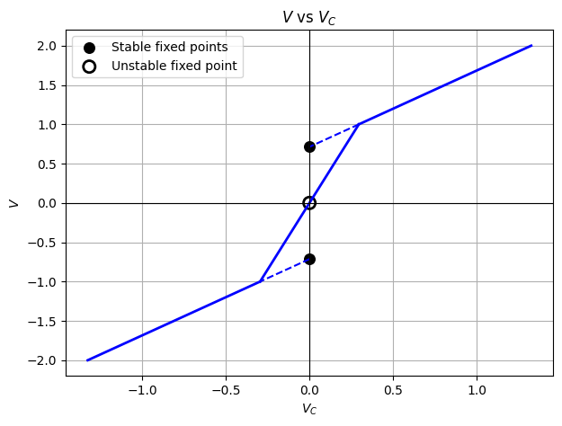
To better see what happens to a trajectory, we can plot $V_{C}$ vs $V$ vs $I_L$ by simply extending the segments into planes for $I_L$ because the inductor current has no constraint. Try rotating it and zooming in to see how this trajectory, a limit cycle, moves across it!
If a trajectory starts in the outer segment, it starts to move toward the stable fixed point in a decaying spiral. These fixed points in the outer segments are also called virtual fixed points, because they only exist when the trajectory is on the outer segment and yet the trajectory can never reach it because it is limited to the $V$ versus $V_C$ curve.
By the time the trajectory almost completes a loop, it crosses into the middle plane where the unstable node pushes the trajectory outward until it ends up in the other outer segment and repeats the cycle to form a loop.
Another case occurs for $G < |G_{a}|$ where the $V_C$ versus $V$ becomes a "fold":
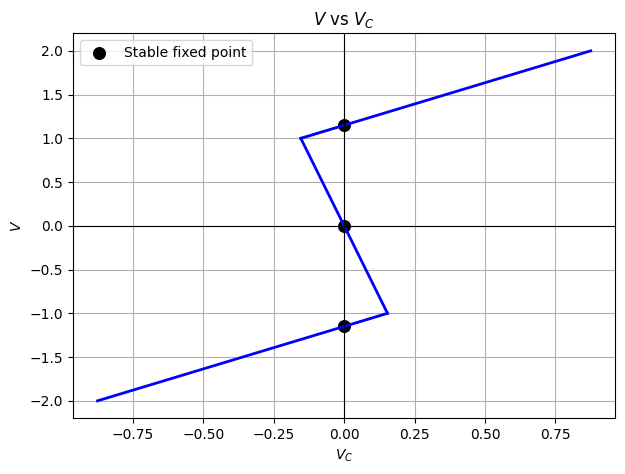
Similar to the previous case, the fixed points occur where the curve intersects the $V_C$ axis. With $G_a > 0$ and $G_b > 0$, all three fixed points are stable. A trajectory starting in the top region will moves towards the top stable equilibrium point, but may reach the edge of the plan before it does so and jump down to the other plane, looping around to form a limit cycle.
This effect cannot be modeled by our current circuit with one capacitor because at $V_C = 0$, $V_C$ can be three possible values. We can fix this by adding a small parastic capacitance across the negative impedance converter so that $V$ can now change with time. After renaming $V_C \to V_2$, and $V \to V_1$, the circuit becomes:
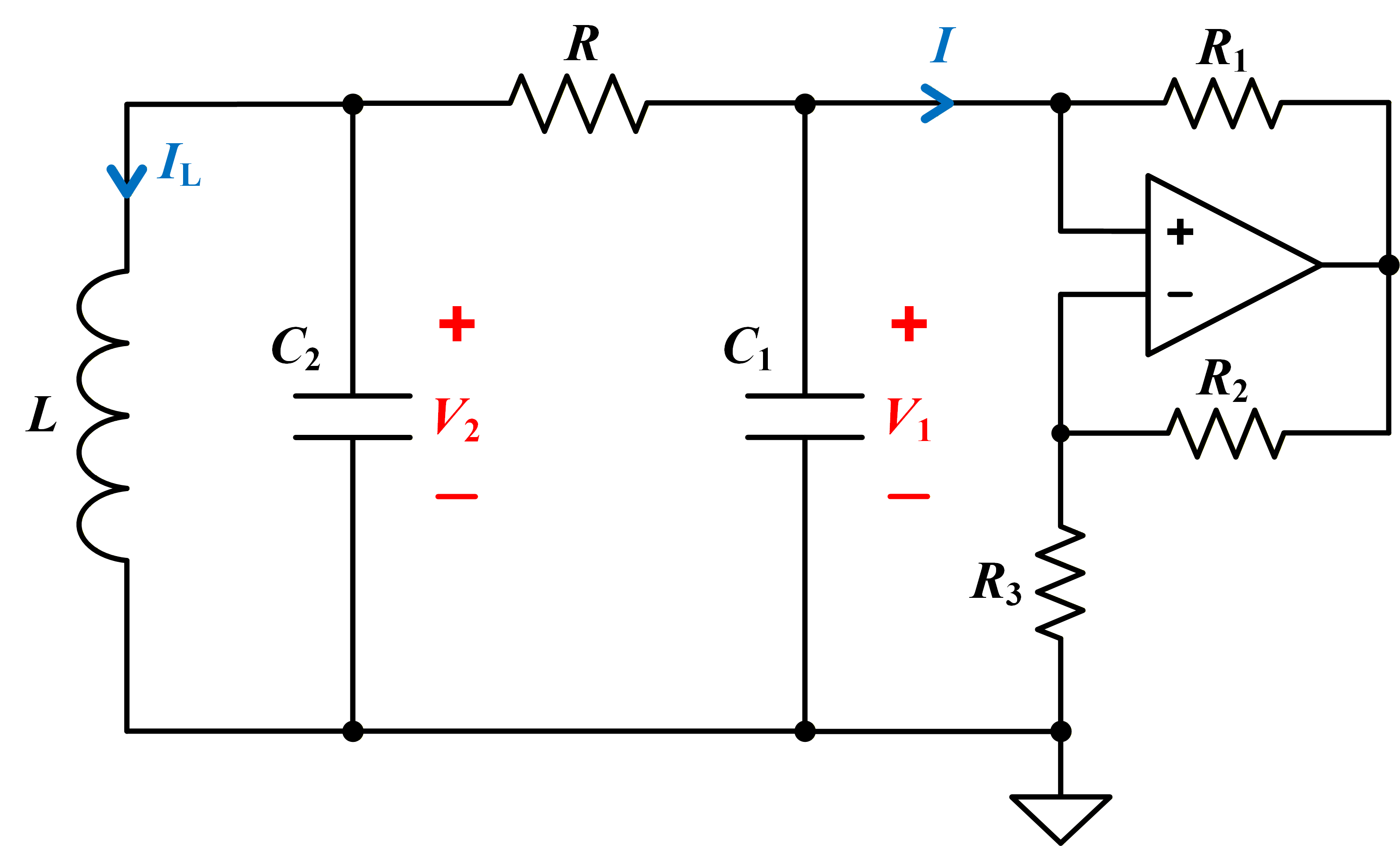
$$\begin{aligned} \dot{V}_1 &= [G(V_2 - V_1) - I(V_1)]/C_1, \\\dot{V}_2 &= [I_L - G(V_2 - V_1)]/C_2, \\\dot{I}_L &= -V_2/L. \end{aligned}$$
The fixed points of the middle point is:
$$(V_{1}, V_{2}, I_{L}) = (0,0,0)$$
And the fixed points of the outer segments are:
$$P_{+,-} = (V_{1}, V_{2}, I_{L}) =(\pm \frac{G(G_b - G_a)E}{G + G_b}, 0, \pm \frac{(G_b - G_a)E}{G + G_b})$$
And the characteristic equation for finding the eigenvalues is now a cubic, since this is a three-dimensional system:
\[\lambda^3+\left(\frac{G}{C_2}+\frac{G+G_a}{C_1}\right)\lambda^2+\left(\frac{GG_a}{C_1C_2}+\frac{1}{LC_2}\right)\lambda+\frac{G+G_a}{LC_1C_2}=0\]
We'll pick numerical values instead of solving this algebraically. For parameters $C_1= 10nF$, $C_2 = 100nF$, $L = 18mH$, $G_a= -757\,\mu\mathrm{S}$, $G_b = -409\,\mu\mathrm{S}$, $E= 1V$, $G=550\,\mu\mathrm{S}$, the inner-region fixed point has eigenvalues:
\[\lambda_1 \approx 26413,\qquad \lambda_{2,3}\approx -5606 \pm j\,20098,\]
and the outer-region fixed points have eigenvalues
\[\lambda_1 \approx -21323,\qquad \lambda_{2,3}\approx 861 \pm j\,19147.\]
When we add the capacitor $C_1$, the system becomes three-dimensional, and each fixed point now has three eigenvalues (one real and a complex conjugate pair). This new fixed point is called a saddle focus, where the trajectories are repelled along one direction determined by the eigenvector corresponding to $\lambda_{1}$, while simultaenously being attracted on a 2D plane formed by the span of the eigenvectors corresponding to $\lambda_{2,3}$.

Route to Chaos
At this point, we have simply designed and modeled a practical RLC oscillator circuit, and found that it had 3 saddle cycles but Chua figured out a way to make it chaotic by satisfying Shilnikov's theorem. What this theorem says in a nutshell is that if you can fold back the trajectory that is pushed out of the plane to join back on itself (a homoclinic loop), the system will have chaotic solutions because it creates the stretching and folding motion needed to create the fractal microstructure of a chaotic attractor.

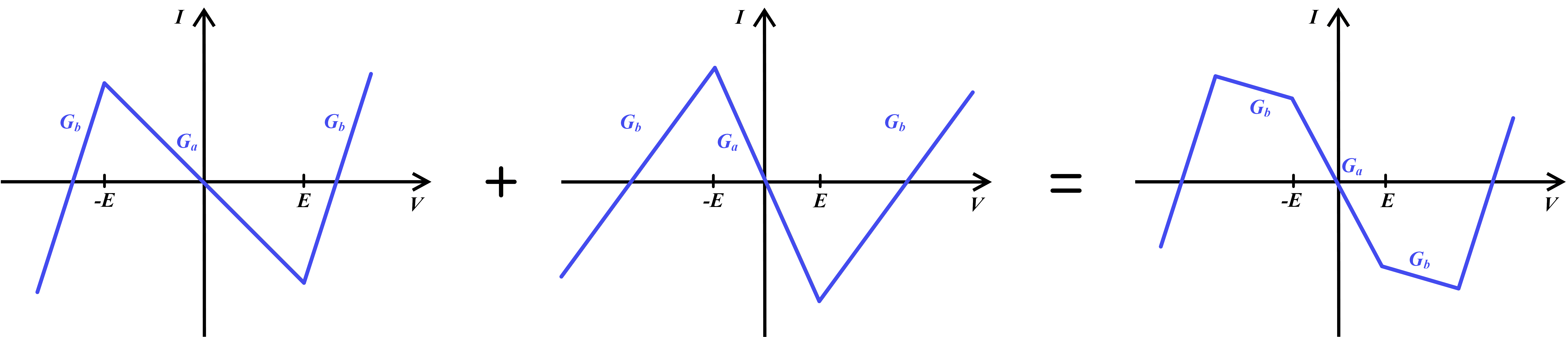
What Chua realized is that Shilnikov's theorem would be satisfied if we switched the polarity of $G_b$ to $G_b < 0$, which can be done by adding another negative impedance converter in parallel with the first one:
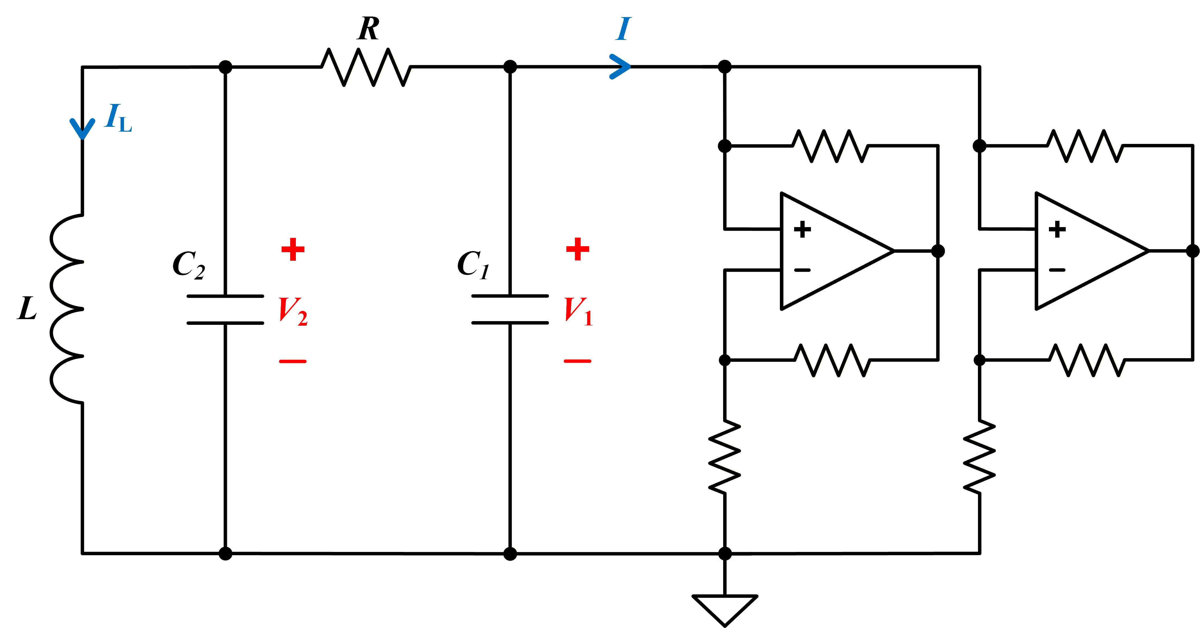
By adding two negative impedance converters, we graphically obtain an I-V curve where $G_a$ and $G_b$ are both negative, until the operational amplifier saturates and becomes a regular resistor.
This leads to the full Chua's circuit equations:
$$\begin{aligned} \dot{V}_1 &= [G(V_2 - V_1) - I(V_1)]/C_1, \\\dot{V}_2 &= [I_L - G(V_2 - V_1)]/C_2, \\\dot{I}_L &= -V_2/L. \end{aligned}$$
The nonlinear resistor is described by the piecewise-linear current-voltage characteristic:
$$I(V) =\begin{cases} G_b V + (G_b - G_a)E, & V \le -E \\ G_a V, & |V| \le E \\ G_b V + (G_a - G_b)E, & V \ge E \end{cases}$$
where $G_a < 0$, but now $G_b < 0$.
Parameters are $C_1 = 10\,\mathrm{nF}$, $C_2 = 100\,\mathrm{nF}$, $L = 18\,\mathrm{mH}$, $G_a = -757\, \mu\mathrm{S}$, $G_b = -409\,\mu\mathrm{S}$, and $E = 1\,\mathrm{V}$, and we will adjust $G$ to see how the system evolves.
For $G = 500\, \mu\mathrm{S}$, the outer fixed points are stable saddle foci (shown by a black dot) with a stable real direction (shown by green arrows along the eigenvector), so any trajectory close to it will spiral into the fixed point.
Furthering increasing $G = 530\,\mu\mathrm{S}$, the outer fixed points undergoes a Hopf bifurcation where the fixed point switches from stable to unstable (shown by an open dot), so a trajectory along the eigenplane spirals outward until it enters the middle segment. The real eigenvector of the middle segment is unstable (red arrows) so it will then push the trajectory is pushed back into outer segment, forming a loop.
If $G = 537\,\mu\mathrm{S}$, the returning trajectory gets pushed into a slightly different part of the outer segment and makes two orbits, also called a period-2 limit cycle.
At $G=539\,\mu\mathrm{S}$ it makes four loops (period-4).
And at $G = 550\,\mu\mathrm{S}$ we obtain chaotic behavior, where it no longer repeats its orbit. Here it becomes more clear how Shilinkov's theorem is satisfied because the trajectory spirals outward due to the unstable saddle foci on the outer segment, but then folds on itself because the real eigenvector of the middle segment pushes the trajectory back.
Also notice that the trajectory comes close but never actually touches the middle plane, if it were to, it would spiral into the stable fixed node of the complex plane and cease to oscillate.
At $G = 565\,\mu\mathrm{S}$, the trajectory will occassionally end up of the other side of the middle eigenplane, where the real eigenvector pushes it towards the other outer segment where it repeats its spiral out and creates a double-scroll plot. This middle eigenplane essentially acts as a "knife's edge", it pushes back the trajectory back on one side, but pushes the trajectory forward on the other side.
We can watch this transition happen in an actual circuit when R is reduced:
To summarize, Chua's circuit can be thought of as a modification of a practical RLC circuit with an additional negative impedance converter to modify the type of fixed points to satisfy Shilnikov's theorem. The result is a simple chaotic circuit without the need for any specialized components.

References
1. Kennedy, M. P. (1993a). Three steps to chaos. I. Evolution. IEEE Transactions on Circuits and Systems I: Fundamental Theory and Applications, 40(10), 640–656. [pdf]
2. Kennedy, M. P. (1993b). Three steps to chaos. II. A Chua’s circuit primer. IEEE Transactions on Circuits and Systems I: Fundamental Theory and Applications, 40(10), 657–674. [pdf]
3. Strogatz, S. H. (2015). Nonlinear dynamics and chaos: with applications to physics, biology, chemistry, and engineering. Chapman and Hall/CRC. [pdf]
